こんにちは。takapy(@takapy0210)です。
本エントリは言語処理100本ノック2020の7章を解いてみたので、それの備忘です。
簡単な解説をつけながら紹介していきます。
コードはGithubに置いてあります。
第7章: 機械学習
単語の意味を実ベクトルで表現する単語ベクトル(単語埋め込み)に関して,以下の処理を行うプログラムを作成せよ.
- 60. 単語ベクトルの読み込みと表示
- 61. 単語の類似度
- 62. 類似度の高い単語10件
- 63. 加法構成性によるアナロジー
- 64. アナロジーデータでの実験
- 65. アナロジータスクでの正解率
- 66. WordSimilarity-353での評価
- 67. k-meansクラスタリング
- 68. Ward法によるクラスタリング
- 69. t-SNEによる可視化
60. 単語ベクトルの読み込みと表示
"""
60. 単語ベクトルの読み込みと表示
Google Newsデータセット(約1,000億単語)での学習済み単語ベクトル(300万単語・フレーズ,300次元)をダウンロードし,
”United States”の単語ベクトルを表示せよ.ただし,”United States”は内部的には”United_States”と表現されていることに注意せよ.
"""

from gensim.models import KeyedVectors


if __name__ == "__main__":
    # ref. https://radimrehurek.com/gensim/models/word2vec.html#usage-examples
    model = KeyedVectors.load_word2vec_format('./GoogleNews-vectors-negative300.bin.gz', binary=True)
    print(model['United_States'])
実行結果
[-3.61328125e-02 -4.83398438e-02  2.35351562e-01  1.74804688e-01
 -1.46484375e-01 -7.42187500e-02 -1.01562500e-01 -7.71484375e-02
 ......
 -8.49609375e-02  1.57470703e-02  7.03125000e-02  1.62353516e-02
 -2.27050781e-02  3.51562500e-02  2.47070312e-01 -2.67333984e-02]
61. 単語の類似度
"""
61. 単語の類似度
“United States”と”U.S.”のコサイン類似度を計算せよ.
"""

from gensim.models import KeyedVectors


if __name__ == "__main__":
    # ref. https://radimrehurek.com/gensim/models/word2vec.html#usage-examples
    model = KeyedVectors.load_word2vec_format('./GoogleNews-vectors-negative300.bin.gz', binary=True)
    print(model.similarity('United_States', 'U.S.'))
実行結果
0.73107743
62. 類似度の高い単語10件
"""
62. 類似度の高い単語10件
“United States”とコサイン類似度が高い10語と,その類似度を出力せよ.
"""

from gensim.models import KeyedVectors


if __name__ == "__main__":
    # ref. https://radimrehurek.com/gensim/models/word2vec.html#usage-examples
    model = KeyedVectors.load_word2vec_format('./GoogleNews-vectors-negative300.bin.gz', binary=True)
    print(model.most_similar('United_States', topn=10))
most_similar関数で類似度が高いTopN個の単語を取得できます。
以下の結果を見る限り、typoが多いようです。
実行結果
[('Unites_States', 0.7877248525619507),
('Untied_States', 0.7541370987892151),
('United_Sates', 0.7400724291801453),
('U.S.', 0.7310774326324463),
('theUnited_States', 0.6404393911361694),
('America', 0.6178410053253174),
('UnitedStates', 0.6167312264442444),
('Europe', 0.6132988929748535),
('countries', 0.6044804453849792), ('Canada', 0.601906955242157)]
63. 加法構成性によるアナロジー
実行結果を見ると、Greece(ギリシャ)がTOPにきており、直感的に良いベクトルが計算できていそうです。
"""
63. 加法構成性によるアナロジー
“Spain”の単語ベクトルから”Madrid”のベクトルを引き,”Athens”のベクトルを足したベクトルを計算し,
そのベクトルと類似度の高い10語とその類似度を出力せよ
"""

from gensim.models import KeyedVectors


if __name__ == "__main__":
    # ref. https://radimrehurek.com/gensim/models/word2vec.html#usage-examples
    model = KeyedVectors.load_word2vec_format('./GoogleNews-vectors-negative300.bin.gz', binary=True)
    print(model.most_similar(positive=['Spain', 'Athens'], negative=['Madrid'], topn=10))
実行結果
[('Greece', 0.6898480653762817),
 ('Aristeidis_Grigoriadis', 0.560684859752655),
 ('Ioannis_Drymonakos', 0.5552908778190613),
 ('Greeks', 0.545068621635437),
 ('Ioannis_Christou', 0.5400862097740173),
 ('Hrysopiyi_Devetzi', 0.5248445272445679),
 ('Heraklio', 0.5207759737968445),
 ('Athens_Greece', 0.516880989074707),
 ('Lithuania', 0.5166865587234497),
 ('Iraklion', 0.5146791338920593)]
1つ疑問に思ったこととして、ベクトルを別で計算してmost_similarで見てみると上記と結果が違いました。
これはなぜだろう...
vec = model['Spain'] - model['Madrid'] + model['Athens']
print(model.most_similar([vec], topn=10))
実行結果
[('Athens', 0.7528455853462219),
('Greece', 0.6685472130775452),
('Aristeidis_Grigoriadis', 0.5495778322219849),
('Ioannis_Drymonakos', 0.5361457467079163),
('Greeks', 0.5351786017417908),
('Ioannis_Christou', 0.5330225825309753),
('Hrysopiyi_Devetzi', 0.5088489055633545),
('Iraklion', 0.5059264302253723),
('Greek', 0.5040615797042847),
('Athens_Greece', 0.5034108757972717)]
64. アナロジーデータでの実験
ここでダウンロードしたアナロジー評価データには、(Athens-Greece, Tokyo-Japan)のように、意味的アナロジーを評価するための組と、(walk-walks, write-writes)のように文法的アナロジーを評価する組が含まれます。
txtファイルの中身をみると分かりますが、gramという単語が入っている行以降は文法的アナロジーを評価する組が含まれているデータになっています。
"""
64. アナロジーデータでの実験
単語アナロジーの評価データをダウンロードし,vec(2列目の単語) - vec(1列目の単語) + vec(3列目の単語)を計算し,
そのベクトルと類似度が最も高い単語と,その類似度を求めよ.求めた単語と類似度は,各事例の末尾に追記せよ.
"""

from gensim.models import KeyedVectors


if __name__ == "__main__":
    # ref. https://radimrehurek.com/gensim/models/word2vec.html#usage-examples
    model = KeyedVectors.load_word2vec_format('./GoogleNews-vectors-negative300.bin.gz', binary=True)

    with open('./questions-words.txt', 'r') as f1, open('./questions-words-add.txt', 'w') as f2:
        for line in f1:  # f1から1行ずつ読込み、求めた単語と類似度を追加してf2に書込む
            line = line.split()
            if line[0] == ':':
                category = line[1]
            else:
                word, cos = model.most_similar(positive=[line[1], line[2]], negative=[line[0]], topn=1)[0]
                f2.write(' '.join([category] + line + [word, str(cos) + '\n']))
65. アナロジータスクでの正解率
"""
65. アナロジータスクでの正解率
64の実行結果を用い,意味的アナロジー(semantic analogy)と文法的アナロジー(syntactic analogy)の正解率を測定せよ.
"""

from gensim.models import KeyedVectors


if __name__ == "__main__":
    # ref. https://radimrehurek.com/gensim/models/word2vec.html#usage-examples
    model = KeyedVectors.load_word2vec_format('./GoogleNews-vectors-negative300.bin.gz', binary=True)

    with open('./questions-words-add.txt', 'r') as f:
        sem_cnt = 0
        sem_cor = 0
        syn_cnt = 0
        syn_cor = 0
        for line in f:
            line = line.split()
            if not line[0].startswith('gram'):
                sem_cnt += 1
            if line[4] == line[5]:
                sem_cor += 1
            else:
                syn_cnt += 1
            if line[4] == line[5]:
                syn_cor += 1

    print(f'意味的アナロジー正解率: {sem_cor/sem_cnt:.3f}')
    print(f'文法的アナロジー正解率: {syn_cor/syn_cnt:.3f}')
66. WordSimilarity-353での評価
相関係数は約0.7くらいになりました。
"""
66. WordSimilarity-353での評価
The WordSimilarity-353 Test Collectionの評価データをダウンロードし,単語ベクトルにより計算される類似度のランキングと,
人間の類似度判定のランキングの間のスピアマン相関係数を計算せよ.
"""

import numpy as np
import pandas as pd
from gensim.models import KeyedVectors
from tqdm import tqdm
tqdm.pandas()


def cos_sim(v1, v2):
    return np.dot(v1, v2) / (np.linalg.norm(v1) * np.linalg.norm(v2))


def calc_cos_sim(row):
    w1v = model[row['Word 1']]
    w2v = model[row['Word 2']]
    return cos_sim(w1v, w2v)


if __name__ == "__main__":

    global model
    # ref. https://radimrehurek.com/gensim/models/word2vec.html#usage-examples
    model = KeyedVectors.load_word2vec_format('./GoogleNews-vectors-negative300.bin.gz', binary=True)
    combined_df = pd.read_csv('combined.csv')
    combined_df['cos_sim'] = combined_df.progress_apply(calc_cos_sim, axis=1)
    spearman_corr = combined_df[['Human (mean)', 'cos_sim']].corr(method='spearman')
    print(f'spearman corr: {spearman_corr}')
実行結果
spearman corr:
               Human (mean)   cos_sim
Human (mean)      1.000000  0.700017
cos_sim           0.700017  1.000000
67. k-meansクラスタリング
"""
67. k-meansクラスタリング
国名に関する単語ベクトルを抽出し,k-meansクラスタリングをクラスタ数k=5として実行せよ.
"""

import numpy as np
import pandas as pd
from gensim.models import KeyedVectors
from sklearn.cluster import KMeans
from tqdm import tqdm
tqdm.pandas()


if __name__ == "__main__":

    # ref. https://www.worldometers.info/geography/alphabetical-list-of-countries/
    countries_df = pd.read_csv('countries.tsv', sep='\t')

    # ref. https://radimrehurek.com/gensim/models/word2vec.html#usage-examples
    model = KeyedVectors.load_word2vec_format('./GoogleNews-vectors-negative300.bin.gz', binary=True)

    # モデルに含まれる国だけを抽出
    conclusion_model_countries = [country for country in countries_df['Country'].tolist() if country in model]
    countries_df = countries_df[countries_df['Country'].isin(conclusion_model_countries)].reset_index(drop=True)

    # 国ベクトルの取得
    countries_vec = [model[country] for country in countries_df['Country'].tolist()]

    # k-meansクラスタリング
    n = 5
    kmeans = KMeans(n_clusters=n, random_state=42)
    kmeans.fit(countries_vec)
    for i in range(n):
        cluster = np.where(kmeans.labels_ == i)[0]
        print(f'cluster: {i}')
        print(countries_df.iloc[cluster]["Country"].tolist())
実行結果
cluster: 0
['Algeria', 'Angola', 'Benin', 'Botswana', 'Burundi', 'Cameroon', 'Chad', 'Comoros', 'Djibouti', 'Egypt', 'Eritrea', 'Ethiopia', 'Gabon', 'Gambia', 'Ghana', 'Guinea', 'Kenya', 'Lesotho', 'Liberia', 'Libya', 'Madagascar', 'Malawi', 'Mali', 'Mauritania', 'Morocco', 'Mozambique', 'Namibia', 'Niger', 'Nigeria', 'Rwanda', 'Senegal', 'Somalia', 'Sudan', 'Tanzania', 'Togo', 'Tunisia', 'Uganda', 'Yemen', 'Zambia', 'Zimbabwe']
cluster: 1
['Australia', 'Bahamas', 'Bahrain', 'Bangladesh', 'Barbados', 'Belize', 'Bhutan', 'Brunei', 'Cambodia', 'Dominica', 'Fiji', 'Grenada', 'Guyana', 'Indonesia', 'Jamaica', 'Kiribati', 'Laos', 'Malaysia', 'Maldives', 'Mauritius', 'Micronesia', 'Nauru', 'Nepal', 'Oman', 'Palau', 'Philippines', 'Qatar', 'Samoa', 'Seychelles', 'Singapore', 'Suriname', 'Thailand', 'Tonga', 'Tuvalu', 'Vanuatu']
cluster: 2
['Afghanistan', 'Argentina', 'Bolivia', 'Brazil', 'Canada', 'Chile', 'China', 'Colombia', 'Cuba', 'Ecuador', 'Guatemala', 'Haiti', 'Honduras', 'India', 'Iraq', 'Japan', 'Jordan', 'Kuwait', 'Lebanon', 'Mexico', 'Mongolia', 'Nicaragua', 'Pakistan', 'Panama', 'Paraguay', 'Peru', 'Uruguay', 'Venezuela', 'Vietnam']
cluster: 3
['Armenia', 'Azerbaijan', 'Belarus', 'Georgia', 'Iran', 'Israel', 'Kazakhstan', 'Kyrgyzstan', 'Moldova', 'Russia', 'Syria', 'Tajikistan', 'Turkey', 'Turkmenistan', 'Ukraine', 'Uzbekistan']
cluster: 4
['Albania', 'Andorra', 'Austria', 'Belgium', 'Bulgaria', 'Croatia', 'Cyprus', 'Denmark', 'Estonia', 'Finland', 'France', 'Germany', 'Greece', 'Hungary', 'Iceland', 'Ireland', 'Italy', 'Latvia', 'Liechtenstein', 'Lithuania', 'Luxembourg', 'Malta', 'Monaco', 'Montenegro', 'Netherlands', 'Norway', 'Poland', 'Portugal', 'Romania', 'Serbia', 'Slovakia', 'Slovenia', 'Spain', 'Sweden', 'Switzerland']
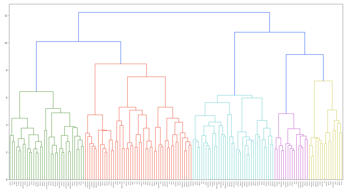
68. Ward法によるクラスタリング
"""
68. Ward法によるクラスタリング
国名に関する単語ベクトルに対し,Ward法による階層型クラスタリングを実行せよ.さらに,クラスタリング結果をデンドログラムとして可視化せよ.
"""

import numpy as np
import pandas as pd
from gensim.models import KeyedVectors
from sklearn.cluster import KMeans
from matplotlib import pyplot as plt
from scipy.cluster.hierarchy import dendrogram, linkage


if __name__ == "__main__":

    # ref. https://www.worldometers.info/geography/alphabetical-list-of-countries/
    countries_df = pd.read_csv('countries.tsv', sep='\t')

    # ref. https://radimrehurek.com/gensim/models/word2vec.html#usage-examples
    model = KeyedVectors.load_word2vec_format('./GoogleNews-vectors-negative300.bin.gz', binary=True)

    # モデルに含まれる国だけを抽出(195ヵ国→155ヵ国になる)
    conclusion_model_countries = [country for country in countries_df['Country'].tolist() if country in model]
    countries_df = countries_df[countries_df['Country'].isin(conclusion_model_countries)].reset_index(drop=True)

    # 国ベクトルの取得
    countries_vec = [model[country] for country in countries_df['Country'].tolist()]

    # Ward法によるクラスタリング
    Z = linkage(countries_vec, method='ward')
    dendrogram(Z, labels=countries_df['Country'].tolist())

    plt.figure(figsize=(15, 5))
    plt.show()
実行結果
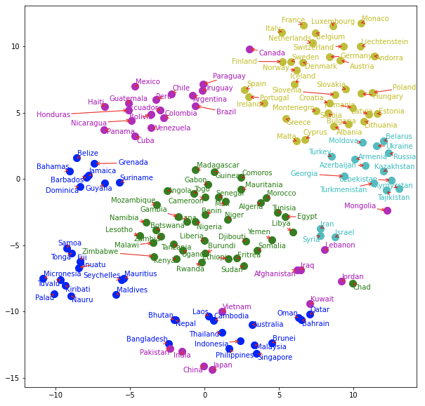
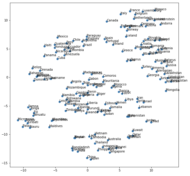
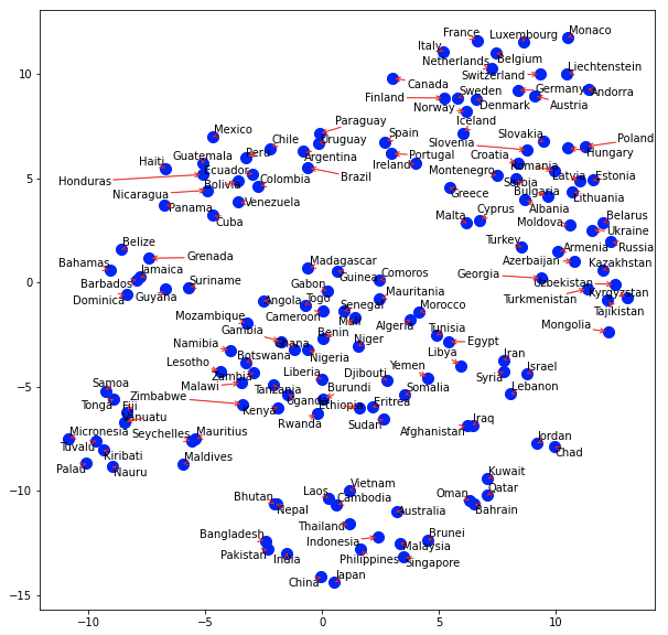
69. t-SNEによる可視化
通常の可視化と、adjust_text*1を用いてちょっと見やすくした可視化を比較してみました。
最後に前項で行ったクラスタ情報で色分けもしています。それなりに良い圧縮ができていそうです。
"""
69. t-SNEによる可視化
ベクトル空間上の国名に関する単語ベクトルをt-SNEで可視化せよ.
"""

import numpy as np
import pandas as pd
from gensim.models import KeyedVectors
from sklearn.cluster import KMeans
from sklearn.manifold import TSNE
from matplotlib import pyplot as plt
from adjustText import adjust_text


if __name__ == "__main__":

    # ref. https://www.worldometers.info/geography/alphabetical-list-of-countries/
    countries_df = pd.read_csv('countries.tsv', sep='\t')

    # ref. https://radimrehurek.com/gensim/models/word2vec.html#usage-examples
    model = KeyedVectors.load_word2vec_format('./GoogleNews-vectors-negative300.bin.gz', binary=True)

    # モデルに含まれる国だけを抽出(195ヵ国→155ヵ国になる)
    conclusion_model_countries = [country for country in countries_df['Country'].tolist() if country in model]
    countries_df = countries_df[countries_df['Country'].isin(conclusion_model_countries)].reset_index(drop=True)

    # 国ベクトルの取得
    countries_vec = [model[country] for country in countries_df['Country'].tolist()]

    # 圧縮
    tsne = TSNE(random_state=42, n_iter=15000, metric='cosine')
    embs = tsne.fit_transform(countries_vec)

    # プロット
    plt.figure(figsize=(10, 10))
    plt.scatter(np.array(embs).T[0], np.array(embs).T[1])
    for (x, y), name in zip(embs, countries_df['Country'].tolist()):
        plt.annotate(name, (x, y))
    plt.show()

    # adjust_textを用いてちょっとみやすくプロット
    texts = []
    fig, ax = plt.subplots(figsize=(10, 10))
    for x, y, name in zip(np.array(embs).T[0], np.array(embs).T[1], countries_df['Country'].tolist()):
        ax.plot(x, y, marker='o', linestyle='', ms=10, color='blue')
        plt_text = ax.annotate(name, (x, y), fontsize=10, color='black')
        texts.append(plt_text)
    adjust_text(texts, arrowprops=dict(arrowstyle='->', color='red'))
    plt.show()

    # クラスタごとに色分けして出力
    n = 5
    kmeans = KMeans(n_clusters=n, random_state=42)
    kmeans.fit(countries_vec)
    countries_df.loc[:, 'cluster'] = kmeans.labels_
    texts = []
    fig, ax = plt.subplots(figsize=(10, 10))
    for x, y, name, cluster in zip(np.array(embs).T[0], np.array(embs).T[1],
                                   countries_df['Country'].tolist(), countries_df['cluster'].tolist()):
        if cluster == 0:
            ax.plot(x, y, marker='o', linestyle='', ms=10, color='g')
            plt_text = ax.annotate(name, (x, y), fontsize=10, color='g')
        elif cluster == 1:
            ax.plot(x, y, marker='o', linestyle='', ms=10, color='b')
            plt_text = ax.annotate(name, (x, y), fontsize=10, color='b')
        elif cluster == 2:
            ax.plot(x, y, marker='o', linestyle='', ms=10, color='m')
            plt_text = ax.annotate(name, (x, y), fontsize=10, color='m')
        elif cluster == 3:
            ax.plot(x, y, marker='o', linestyle='', ms=10, color='c')
            plt_text = ax.annotate(name, (x, y), fontsize=10, color='c')
        else:
            ax.plot(x, y, marker='o', linestyle='', ms=10, color='y')
            plt_text = ax.annotate(name, (x, y), fontsize=10, color='y')
        texts.append(plt_text)
    adjust_text(texts, arrowprops=dict(arrowstyle='->', color='r'))
    plt.show()
実行結果
青色とピンク色のクラスタが若干ばらついていますが、それ以外は良さそうです。